|
If you ever had a need to show the details for one section of a hierarchy, but not all, hopefully this post will do the trick. In this example we will use Superstore data to show the Sub-Category details of one Category, but not the other two.
You will need 2 columns, one for the overall Category and one for the details. Your data may already have a column that has a lower grain of data for some records, but not others. A business example could be the"Sales" line is only total sales, but for "Costs" we also have a secondary breakout by Cost of Goods Sold, Marketing Costs and Admin Costs. For Sales we just want to show total sales and for cost we want to show total costs AND the breakouts by cost type. For this example we will use a table, but this also applies to bar charts and other visuals: 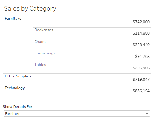
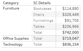
As you can see in the chart above, in addition to showing each Category totals, we show the details for Furniture.
As mentioned above, I created a column in the superstore data that only showed the sub-category based on a parameter. 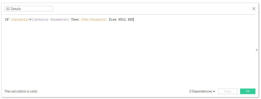
Step 1: Bring the two fields into the view. You will get something that shows the totals for the amounts without any details, and the detailed breakout (without a total) for the other category.
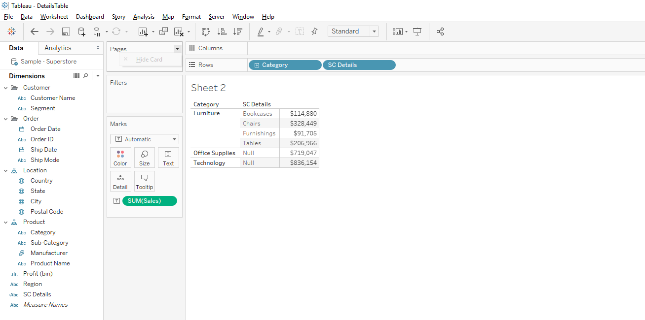
Step 2: Add subtotals to your view. You now have a total amount for each category. Notice, the amounts where there are no details is now unnecessarily duplicated because subtotals are shown for all categories.
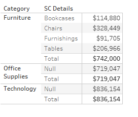
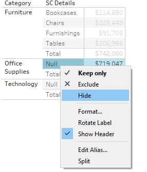
Step 3: Hide the value NULL. This will remove the original data point and only leave to subtotal. While you cannot selectively show / hide subtotals (unfortunately) this will dynamically hide all instances where there are no details in the second column leaving you with the amount shown once.
Step 4: In the Format Pane remove the word "Total" from the label making it blank. This will clear the "Total" label from the second column without details, leaving only the details labeled.
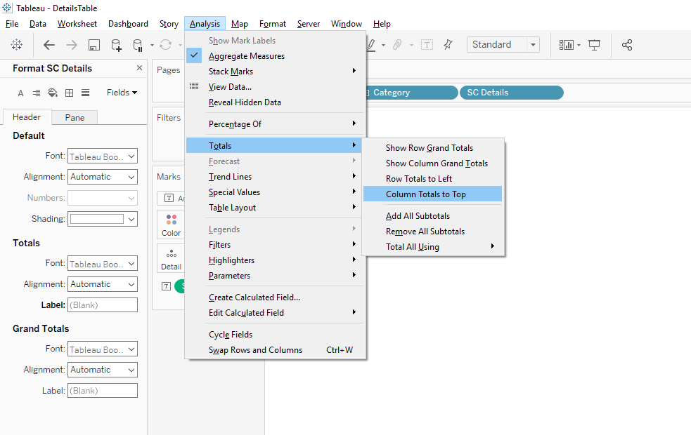
Under Analysis tab at the top, choose to show totals at the top. 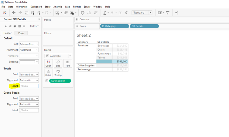
All that is left now is some formatting. I chose to remove row banding, column dividers and left the row dividers. Since all your Category amounts are technically subtotals they will be bold and you can control their format separately from the details.
Thanks for reading! Corey 
2 Comments
I've recently stumbled on this #TinyTableauTip and wanted to share it with the world. Do you ever find yourself needing to switch a dimension on a worksheet, but end up losing all your formatting? Maybe you duplicate a sheet but need to change the dimension? Look no further. Let's set the stage and format our worksheet:  We have sorted our dimension (sub-category) descending based on sales and increased the size of the Sub-Categories. Now if we simply want to swap Sub-Category out for State, we could drag State ontop of Sub-Category to replace it, but you will see, it clears the formatting and we lose the sort:  Now, rather than dragging a pill to replace Sub-Category, simply double click on the Sub-Category pill in the rows window. Now within the pill type "State" to replace Sub-Category. This will preserve any formatting changes and the sort:  The reason I think this works is because the formatting must be fixed to the pill, and by in-line editing and changing the dimension in the pill, you keep your formatting.
Thanks for reading! Corey 
Set Actions Part Two! In this example we use Set Actions to specify a date range. We will then use the set to highlight color and filter other graphs on the dashboard.
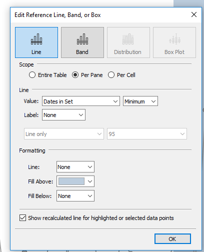
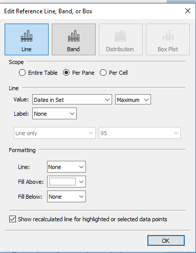
Tip 1: Highlighting a timeline using reference line 1) Create a calculated field based on the level of desired detailed for your timeline – in this case I used month and year: [Month / Year]: DATETRUNC('month', [Order Date]) 2) Create a set based on the new field above 3) Create a second calculated field keeping only the date values in the set: [Dates in Set]: IF [Date Set] Then [Month / Year] END 4) Add the new calculated field, Dates in Set, to the circle mark, to not break your path. 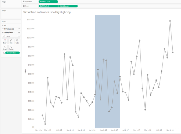
5) Add two reference lines: min(Dates in Set) and max(Dates in Set).
Color above the min reference line with a color, color above the max reference line to match the background (in this case, white).
Tip 2: Color bars based on values in the set
Simply the set (Date Set) to the color shelf 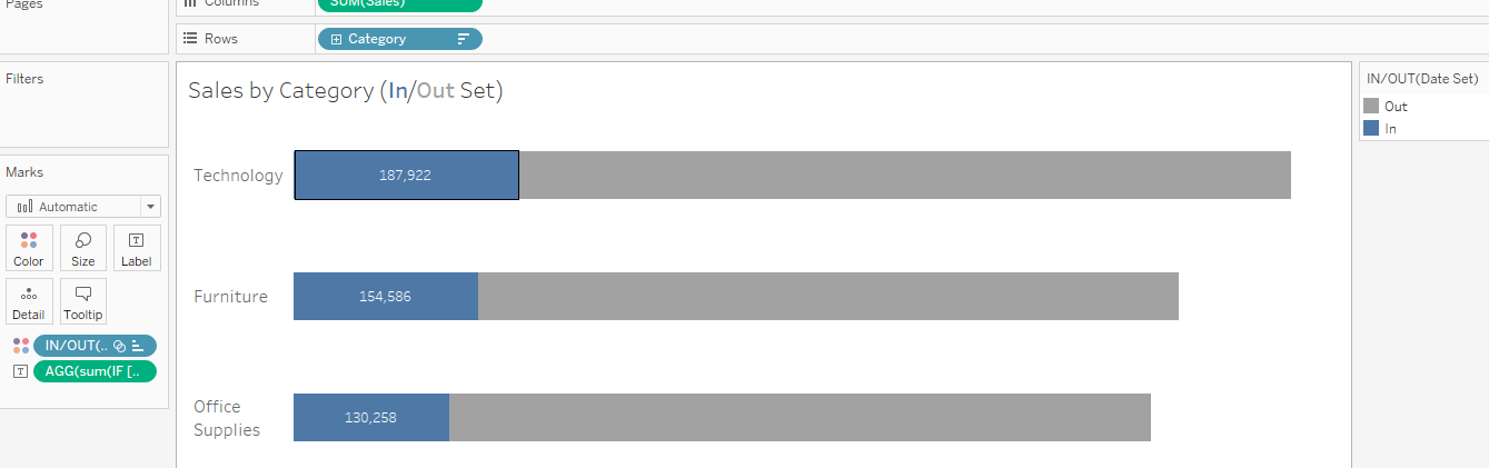
Tip 3: Filter based on values on a set
Drag the set to the filter menu to keep values “IN” set 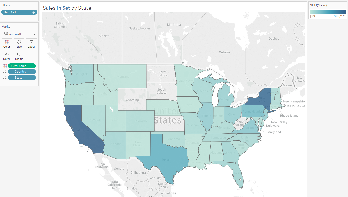
As you highlight new ranges of data on your timeline, your bars and map with update to represent the dates in your range. By using the option to Keep Set Actions, you can deselect you the marks on your timeline, and interact elsewhere on the dashboard, but your set range will remain – and your audience will know the range because the timeline stays shaded.
Thanks for reading – let me know if you have questions! 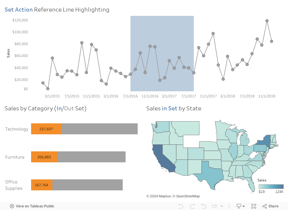
Devs on stage was awesome! While many things caught my eye, as someone who has hacked together click-and-drill dashboards using traditional Tableau actions, I immediately wanted to recreate the tree map click-and-drill demo. Soooo, let’s do it.
Turns out it is not as difficult as one may expect, and it requires only two calculated fields and two sets. Best of all, it requires no LOD calcs. In this case, we are going to build a tree map based on superstore data that drills from Category > Sub-category > Product. We will use the category field as it appears in the data because it is at the highest level. 1) Create a set based on the category field. 2) Create a calculated field that tests what is in the set above: If the category matches the value in the set above, return the sub-category otherwise return category. Once a category has been selected on the dashboard, it changes the level of detail for only the select category (the one in the set) to sub-category – “drilling-down.” CALC: IF [Cat Set] then [Sub-Category] ELSE [Category] END 3) Create a second set on the new dynamic subcategory field 4) Create the second calculated field which tests two conditions:
5) Now create a worksheet with Category, Dynamic SubCat and Dynamic Product in the details. 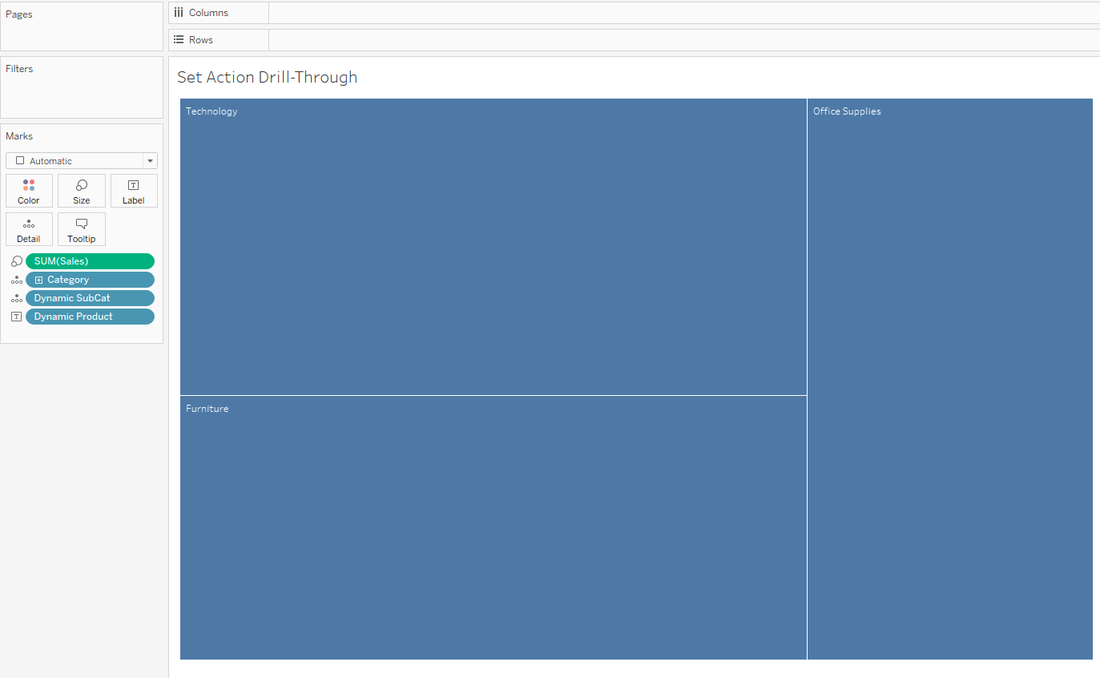
6) Add the worksheet to the dashboard and add 2 Set Actions to run on select and remove all values from set when cleared. The first set action will address the Cat Set and the second the SC Set.
Optional: You can add dynamic product to labels, but ensure you keep the order on your marks card Category > Dynamic SubCat > Dynamic Product (label). You are set -- drill away! Let me know if you have questions. 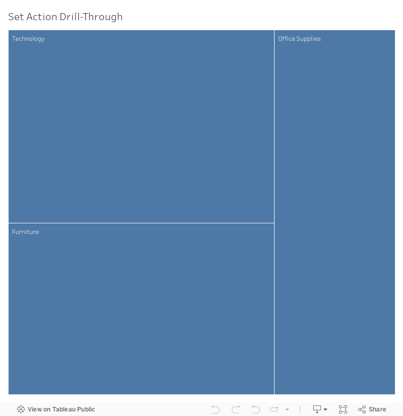
Background: I recently had the idea that I wanted to track the Sixers likelihood to make the playoffs. The original plan was to create a model by testing factors such as strength of schedule (SOS) played, SOS remaining, current record, and others keeping those which were significant. After doing some research I found BasketballReference.com has completed a similar exercise and created an award-winning model. This sparked a new question: could I automatically retrieve what BasketballReference is predicating each day and track how the Sixers’ odds change?
I determined there were three main things that I needed to do:
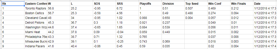
1. Fetching the Data To create something hands-off I knew I would be calling on Google Sheets. I have used the Google’s IMPORTHTML() function in the past so this part was not too bad. Since the table is relatively fixed (there will not be new teams—rows – added) I was able to simply use the function twice to pull the data from the Eastern Conference table and the Western Conference table. =IMPORTHTML("https://www.basketball-reference.com/friv/playoff_prob.html","table",1) 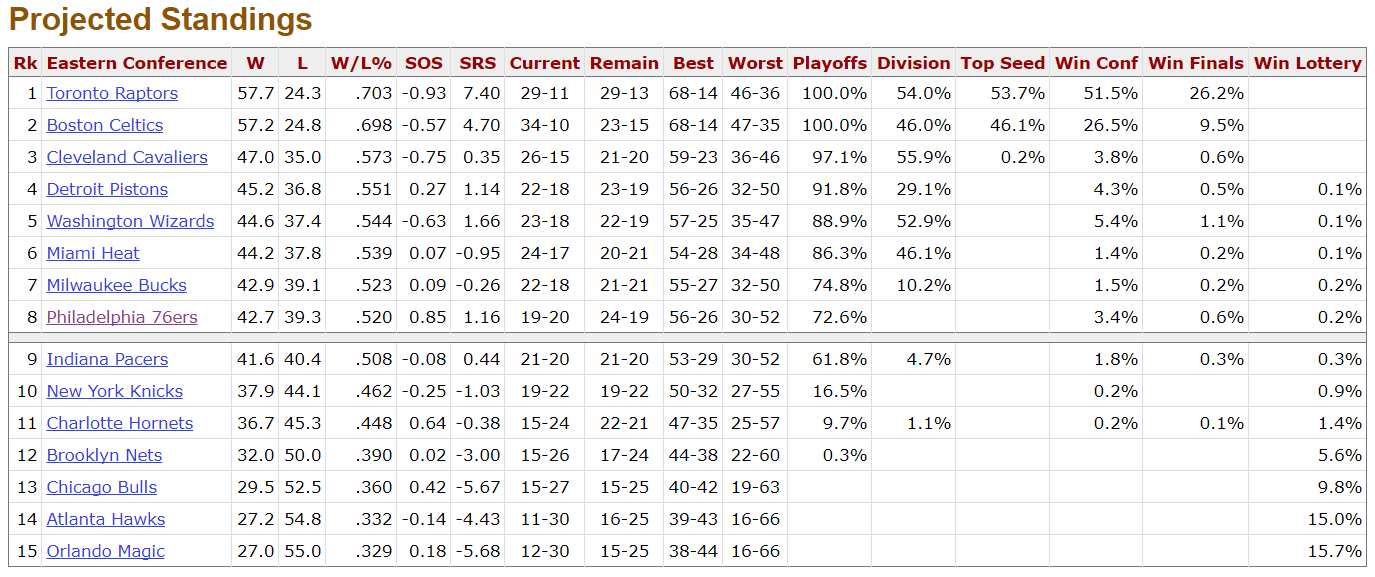
Table 1 from BasketballReference
=IMPORTHTML("https://www.basketball-reference.com/friv/playoff_prob.html","table",2) 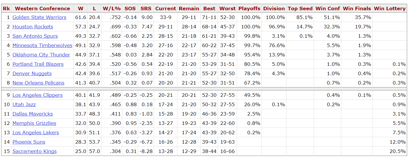
Table 2 from BasketballReference
I then added a few additional columns after the table. The one that will be important later was the date and time field. By using the function NOW(), when the data is retrieved there will also be a time stamp. 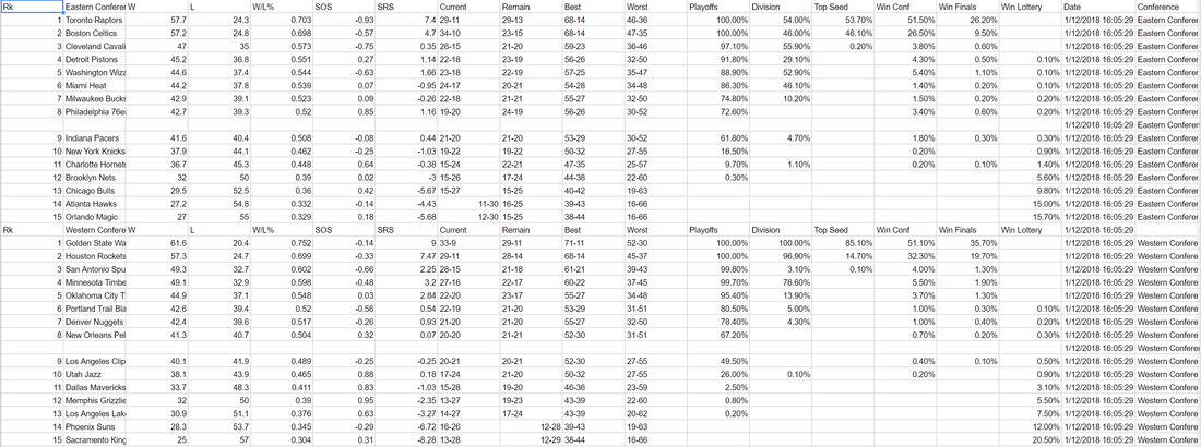
Data from BasketballReference in Google Sheet using ImportHTML function
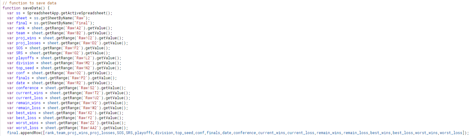
2. Archiving the Data Now that I had the data and a timestamp when the data was pulled, I wanted to move this data to a new sheet so that I could add the results each day. Like Excel with macros, Google Sheets has a feature called Script Editor. I was able find a template to get me started by Ben Collins. In this example, he has a single cell returning a value from the web and created a script to copy the value to the bottom of a running list on the same sheet. The basic premise is to use Google Sheets' variable (var) function to define the cells you wish to copy and use the appendRow() function to add the rows to the bottom of a table. The important change I made to the original example was having the result write to a separate sheet than the original data was found. This is achieved by creating two variables, one defining where to source the data (in this case it is called "Sheet") and one to write the final data to (“Final”). 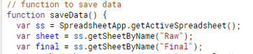
Next simply define which cells need to be copied form the original sheet using the getValue() function. Each new variable will be used in the append rows function to tell Google to copy the value in the reference cell. In the code below, the "sheet" after the equals sign is a reference to the variable we defined above, which allows it to know to get data from the sheet called "Raw" in the workbook.
And with the cells defined, list all your variables from above in the appendRow() function. Note, the final.appendRows is referencing the variable we created above to indicate the data show be placed in the sheet called "Final":

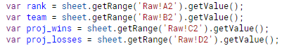
When you run the script, Google Sheets will copy all the values from the specified cells into the next available row in your Final sheet. If you have multiple rows in your source data, like I did, you will need to copy the entire function and change the row number in your script to reference the next row in the Google Sheet (for example change Raw!A2 to Raw!A3. Code Snapshot for one row:
3. Automating the Process
Now let’s make it run by itself. This is fairly easy. We first need to automate the IMPORTHTML function. By creating the following code in the script editor, Google will simply place the what is defined as "cellFunction" in the cells specified (in this case A1 and A18). By placing the function in the cell, it will cause the function to refresh with new data from the site. 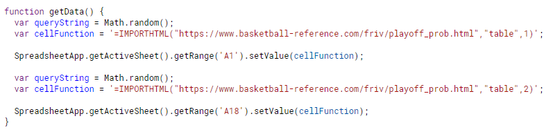
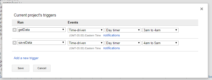
Still in your Script Editor, under the Edit Menu select Current Project Triggers. Here you can tell Google Sheets to run a function automatically based on a "tigger", for example, a certain time (monthly, weekly, daily, hourly, etc.). Note, I made sure to set my getData function to run before the saveData function.
The result? Each day I will have a nice data table that ran overnight with the updated NBA playoff picture.
Time to connect this worksheet to Tableau and get vizzing! I look forward to seeing how you use this function!
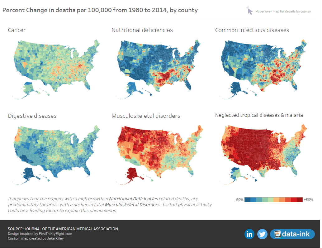
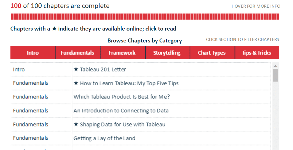
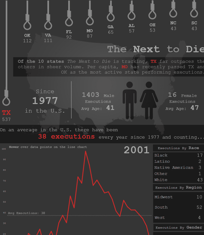
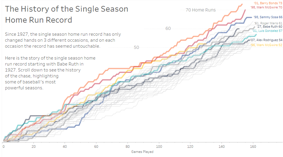
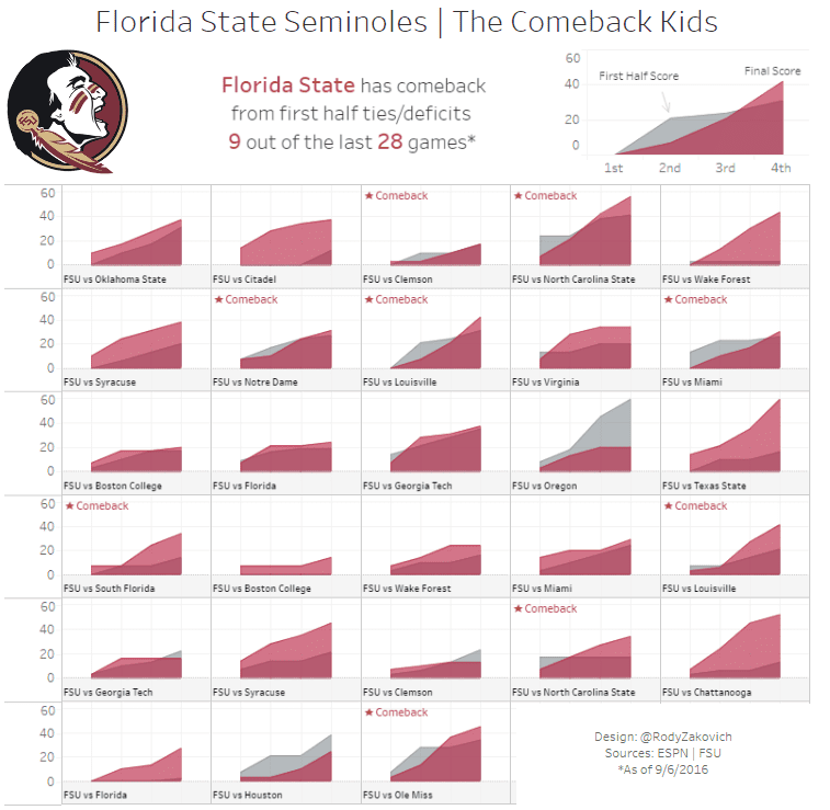
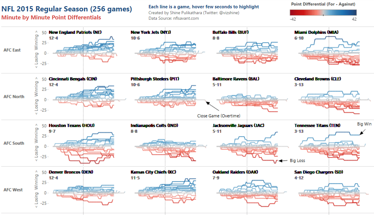
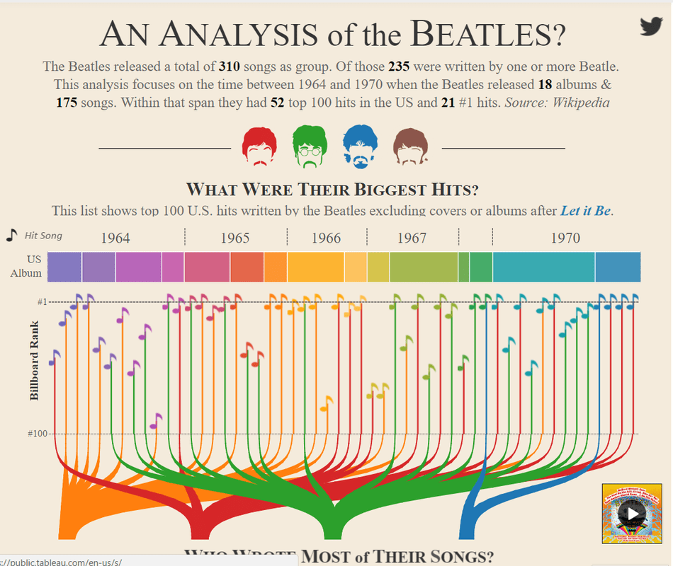
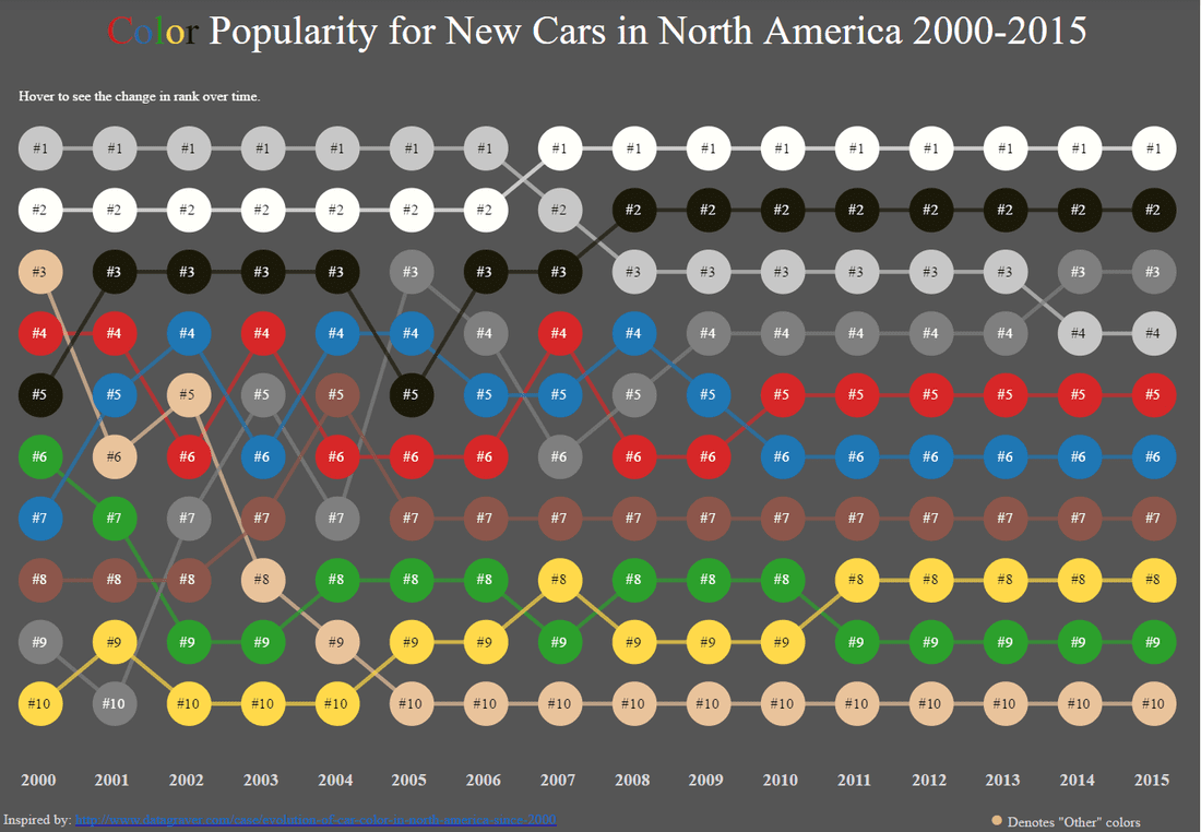
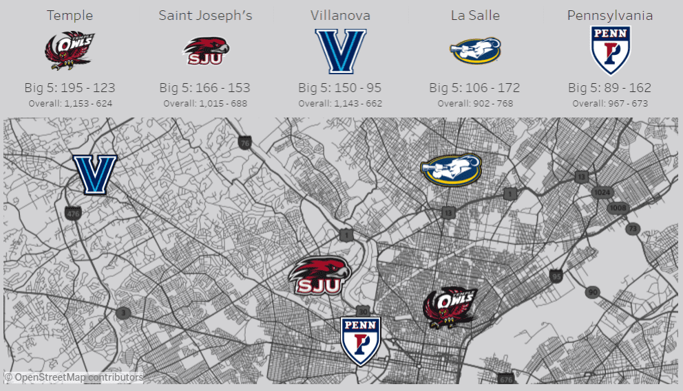
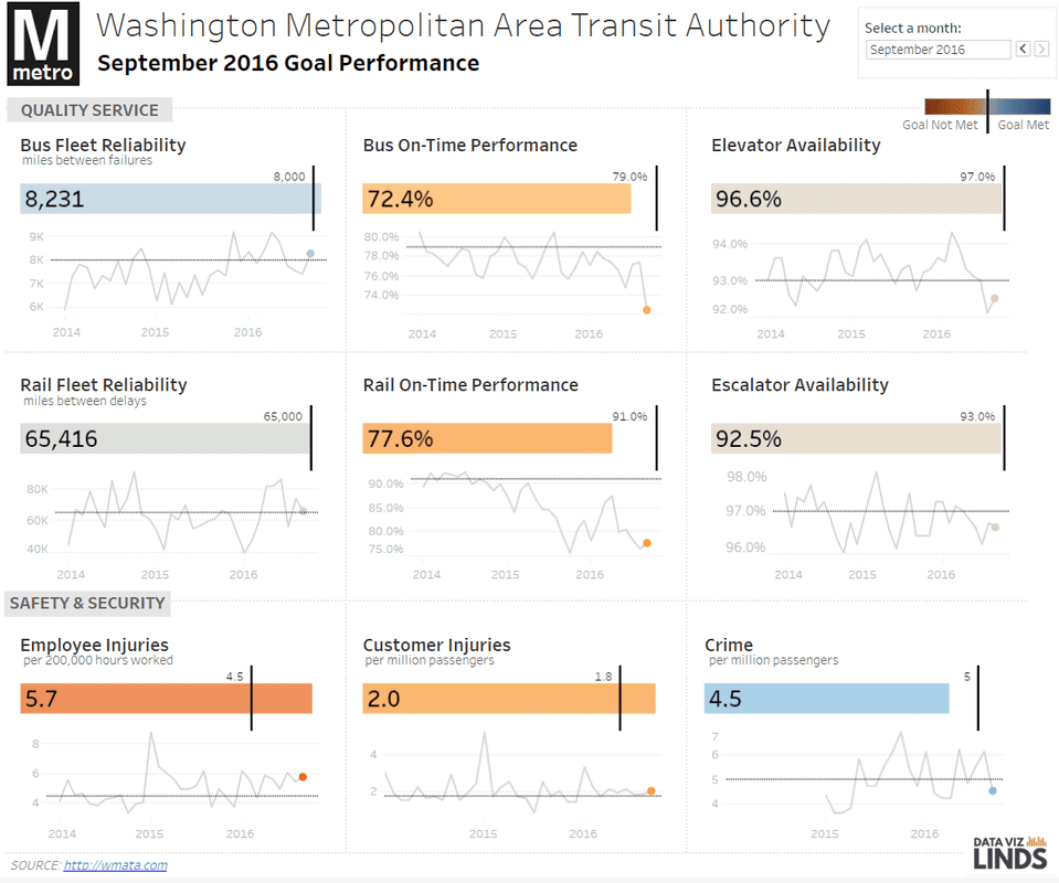
Thanks for reading. Questions? Feel free to reach out on Twitter @coreyj34. Corey Iron Viz! What a challenge. Take all the skills that you have learned through practice and the Public community, sift through your toolbox, and produce an engaging dashboard for the given topic. Getting Started One of my favorite aspects of Iron Viz is that it is an end-to-end process. I start by brainstorming topics and hunting for data. This time, I originally thought the animal option of the animal or plant prompt was more interesting to me. I had ideas of trying to analyze which animals make zoos popular (based on zoo visitations), tracing the descendents of dinosaurs, or examining the history and success of race horses. While I found these topics interesting, I did not feel connected or passionate about any of the topics above. Back to the drawing board. I quickly came around to the topic of the effects of medical cannabis on epilepsy. I had some initial insights into this space-- my little brother has intractable epilepsy – meaning that his epilepsy is not able to be successfully controlled by medicine. I occasionally hear my mom talking about a new study that has shown very promising results using the plant cannabis, but I frankly did not know much about the topic. I figured this was the perfect opportunity to learn. The Design I decided early on in the process that I wanted to infuse a personal touch into my design. One thing I admire about FiveThirthyEight's dashboards is their use of annotations. I thought I would take my own spin on this and use a custom font made from my own handwriting to annotate my dashboard. I used this font to highlight some of my analysis of the data. My original dashboard was a "long and tall" style. The annotations were mixed into the dashboard. While there was a definite narrative, I felt the dashboard was becoming cluttered. I decided to break the main elements of the dashboard apart, and place them into story points. This separation allows each section to focus on a particular element while still within the larger story. I added the notes section in the margins to create the feel of a notebook. My Learnings While you always learn something from practicing and vizzing, here I will categorize my learnings into two major ideas. 1) Viz about something you have passion for. Your analysis will be driven by your curiosity and determination to deliver a product that is useful and informative to others. 2) Do not be afraid to go through multiple iterations and even go back to the drawing board on an idea. While this is not a new learning for me, this Iron Viz did serve as a good reminder. One key to successfully iterating a dashboard is allowing an appropriate amount of time for review. If you are crunched for time, it is likely your first design will be your final. I was able to start this challenge a week ago which gave me time to work on it, put it down, and come back to evaluate my design choices. Most of the main elements remained the same throughout the process, but the iterations in structure, ordering of elements, and additions/removals of supporting elements helped this dashboard greatly. I hope you learn something from my dashboard. Thanks for reading. Corey  In a recent dashboard I used custom shapes to create a 10-star rating scale. I first saw this technique used when looking at a Tableau dashboard of Annual Births in a post by Bora Beran 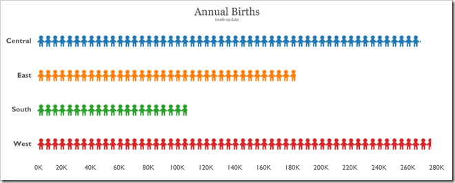 The basic premise is to make custom icons that represent your scale. I made 10 separate custom icons that would represent a filled star from 0.1 to 1.0. This allows you to represent any rating between 0 and 10 (4.1 stars, 6.3 stars, etc).  To make the stars I used PowerPoint. I started with one star that was 1in x 1in. I made the fill transparent and gave it an outline color. I duplicated the star and added a fill color. I overlaid the stars and saved this as “1”. I then began cropping the filled star by .1in and saving each increment as a new image (0.9, 0.8, 0.7, etc). The result is 10 images, each 1/10th more filled than the previous. 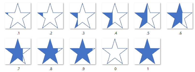 You can now use these custom images in Tableau to represent your rating. By keeping the image transparent, you can change the color using the color mark in Tableau. Let me know if you have any questions! You can download the 10 stars I saved here: LINK. Thanks for reading, Corey  As 2016 winds down, Tableau Public authors have been sharing their favorite dashboards using #VizInReview on Twitter. Here are some of my favorites that have certaintly influenced my work and taught me new skills (in no particular order): Adam Crahen -- Night Biking: You may not even realize it is a Tableau dashboard, built off of actions, Adam integrates Youtube and JS to create a very cool animated dashboard! Josh Tapley & Jake Riley -- Disease Death Rates: Wow, these maps are stunning. Great design and storytelling packed into a very clean dashboard. Ryan Sleeper -- Tableau 201: Have you seen this? A book in a dashboard! The tips and tricks in here are awesome for anyone looking to learn Tableau or hone their skills. Check it out! Pooja Ghandi -- The Next to Die: The design on this dashboard is fantastic. My favorite part is the bar graph perfectly integrated with custom icons to create a striking way to show volume of state executions. Curtis Harris -- This History of the Single Season Home Run Record: The narrative of this dashboard combined with the clean, consistent visuals makes this one of my favorite examples of storytelling this year! This viz was a home run (couldn't resist... sorry). Rody Zakovich -- Florida State Seminoles | The Comeback Kids: I am a sucker for small multiples, but what really tops this one for me are the tooltips. I am sure Adam will approve! Shine Pulikathara -- NFL 2015 Regular Season: Speaking of small multiples, this example by Shine was the first example of small multiples I personally saw in Tableau. I was hooked by Shine's design and almost a year later, I am now hooked on DataViz and Tableau. This one helped kick start it all -- thanks, Shine! Adam McCann -- Beatles Analysis: Published January 2016, it was pretty clear this was going to be at the top of the charts for this year. Almost 770K views later, it is safe to say this data viz has made an impact. Matt Chambers -- Car Color Evolution: My favorite example of a bump chart. This dashboard is clean, engaging and tells a story. It also has attracted many other authors to ReViz it and continue learning new techniques as a result. Lindsey Poulter -- March Madness: You may say I am biased because March Madness is my favorite sporting event, by far, but this viz is elegantly designed with tons of information packed into an engaging, interactive dashboard. Tom O'Hara -- Philadelphia Big 5: Philly basketball. Tom has used some really nice techniques to make his map pop, and incorporated learnings from the community, like Matt's bump chart, into this really cool Big 5 dashboard. Go Hawks! Lindsey Poulter -- MetroVitalSigns: A must for future VOTD, this example of a scorecard is my favorite #MakeoverMonday of the year. I can only imagine how many business applications this design may influence in the future.
How-To: Visualize your ESPN Fantasy Football Data:
This blog post will be focused on how you can use my new Tableau fantasy football dashboard with your own ESPN fantasy football league. Subsquent posts will examine the dashboards within the package, and how I created them in Tableau. Shoutout to Tom O'Hara for pushing me to complete this bootstrap, to Adam Crahen and Ryan Sleeper for the peer reviews of the workbook ,and to Rody Zakovich for help with the arcs in the workbook. This bootstrap is structured to use ESPN fantasy football league. The excel template contains a macro that will streamline the data wrangling process. The macro is set up to format leagues with the positions shown below. The file can be modified to accommodate other league formats, please let me know if you need help! Note, while this package is set up to work with ESPN data, data from other fantasy leagues can use this Tableau workbook if you structure your data in the table format on the “Data” tab of the excel file. 1 – QB 2 – RB 2 – WR 1 – TE 1 – FLEX 1 – D/ST 1 – K 6 – Bench Step 1: Log into your fantasy league and navigate to the ESPN quick box score for the desired week. Step 2: Click on the “show bench” option to see the entire quick box score. Step 3: Highlight the entire box score and copy the data. Step 4: Navigate to the excel template “Dump” tab. Place your cursor on cell A1 and then paste the data, overwriting any existing data. Step 5: Run the macro “BoxCleanandCopy”. Note, this macro will automatically create and delete a temporary sheet in the excel file (Temp_2). When prompted select delete. When the macro is complete, it will automatically take you back to the “Dump” tab. The macro will have added the data to the bottom of the “Data” tab. Step 6: Repeat steps 2-5 for each matchup of the week. Step 7: Navigate to the “Data” tab. Manually add the week number (1,2,3,etc.) to Column “K” and add the number “1” to each row in column “L” (this 1 enables joins for the use of arcs in the workbook). Step 8: Save the excel file and update your Tableau workbook. While this does require a manual copy and paste, it only took about 5 minutes a week for me to update a 12 team league. If anyone was a better way than copy/paste to automate the data collection process from ESPN please reach out. Files to download and screenshot with instructions below. Please feel free to reach out with any questions @CoreyJ34 on Twitter. Files for Download
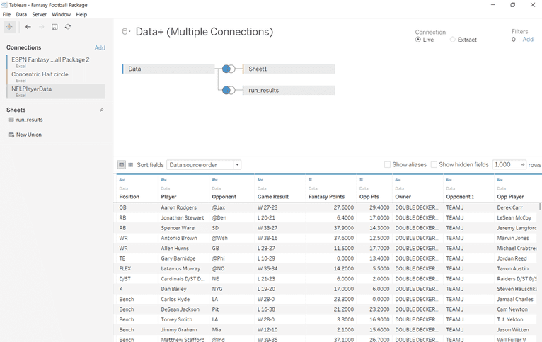
Download the Tableau file and 3 excel files. The Excel file espn fantasy football package is the main data source. The other two files are used to enable some of the visuals, and are joined using left joins. See image below of connection in Tableau.
Visual InstructionsCorey's 2016 Fantasy Football Dashboard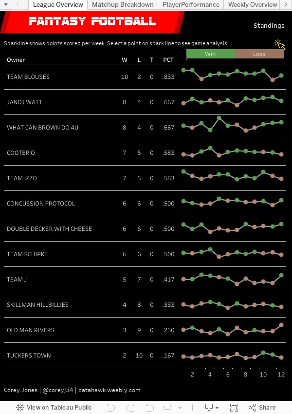
|
AuthorCorey Jones | @coreyj34 Archives
December 2018
Categories |
||||||||||||


 RSS Feed
